Welcome to the homepage for Numerical Analysis (Math 4500/6500)! I will post all the homework assignments for the course on this page. Our text for the course is Cheney and Kincaid, Numerical Mathematics and Computing (seventh edition). If you want to save money and get the 6th edition for a lot less money, you’ll be fine. During Spring 2020, the class meets twice a week at 12:30-1:45 TR in Boyd 322. Office hours are Wednesday 2-5pm in Boyd 448.
Numerical analysis is the art and science of doing mathematics with a computer. This is where you can start to bridge the gap between the formal mathematics that you have learned so far and the mixture of mathematics, statistics, and computation you’ll need for a 21st century job such as working for the algorithms group at StitchFix.
To be really prepared for an industry job, this is the first class in a series which should include
MATH 4500 and MATH 4600 (taken together or in either order)
MATH 4510
MATH 4900 (Optimization with Prof. Hu, Fall 2019)
and
MATH 4900 (Learning from Data with Prof. Adams, Spring 2020)
or
MATH 4050 (Advanced Linear Algebra with Prof. Wang, Spring 2021)
In this class, we will learn the fundamentals of numerical mathematics, covering the basics of numerical arithmetic, finding the roots of equations, and numerical differentiation and integration. We’ll then jump ahead to
Mathematica will be an integral part of the course. Current UGA students can get a copy for your laptop or home computer free of charge by visiting the EITS page here. Some of the homework assignments and projects will require you to write Mathematica programs, and you’ll be completing most of the Introduction to the Wolfram Language online course. Here are some brief notes on Mathematica Programming.
Syllabus and Policies
Please examine the course syllabus. If you think you can get by with this copy, save a tree! Don’t print it out. Please subscribe to the course Google calendar. The course syllabus lists the various policies for the course (don’t miss the attendance policy).
Lecture Notes
Here are links to my lecture notes for the course. Each lecture is usually accompanied by one or more Mathematica notebooks explaining and demonstrating the concepts from class.
- Introduction. What numerical analysis is all about. Mathematica. Examples of problems you can solve with Mathematica.
- Bisection and Newton’s method. Bisection method. Linear convergence. Newton’s method. Proof of Newton theorem on quadratic convergence in 1-d. This lecture comes with demonstrations of the bisection method, Newton’s method, unstable behavior of Newton’s method in one complex variable.
- Newton’s method in n-dimensions. (notes part 1). (notes part 2). Newton-Kantorovich conditions for convergence. Demonstration for inverse kinematics. Ortega’s proof of the NK theorem.
- The secant method. Superlinear convergence of the secant method. Fibonacci numbers! Comparison of Newton’s method and the secant method.
- Interpolation of Data. In this lecture, we discuss the surprisingly difficult and subtle problem of estimating the value of a function between given data points. We include a demonstration of interpolating polynomials.
- Error in Interpolation of Functions. We dig deeper into interpolation errors, discussing interpolating polynomials and nodes and the effect of choice of nodes on interpolation error.
- Everything you didn’t learn about Taylor’s theorem in MATH 3100. General form. Remainder terms.
- Introduction to Error Analysis. Interval Arithmetic. Hickey/Ju/Emden paper on fundamental model.
- Models of computer arithmetic. Fixed and floating point. Demonstrations for linear equations and probability computation.
- Floating point arithmetic. Loss of significance when subtracting nearly equal numbers. Accumulation of roundoff error in repeated addition.
- Details of IEEE floating point on modern computers. Machine Numbers, Conversion to single and double precision floating point numbers (try this with some digits of Pi, such as 3.141592653589793238462643). Here’s the GAO report on the Patriot missile example.
- Estimating Derivatives and Richardson Extrapolation. We give a rigorous procedure, called Richardson extrapolation, for bounding approximation errors.
- Demonstration notebook: symbolic Richardson extrapolation.
- Demonstration notebook: Richardson extrapolation and derivatives.
- Minihomework: Richardson extrapolation.
- Graduate material: Lanczos derivative and minihomework.
- Graduate reading: Lanczos’ Generalized Derivative
- Estimating Derivatives by Polynomial Fitting. We can use interpolating polynomials to estimate derivatives.
- Demonstration Notebook: the approximation for the second derivative.
- Minihomework: Derivatives by Polynomial Interpolation.
- Numerical Integration and the Trapezoid Rule. We now return to Math 2260 and reintroduce our old friend the Trapezoid rule.
- Trapezoid rule videos (3 part playlist). (Notebook)
- Minihomework: The Trapezoid Rule.
- Graduate material: Numerical treatment of improper integrals and minihomework.
- The Romberg integration algorithm is our first really modern integrator.
- Trapezoid rule error video. (Notebook)
- Romberg integration video. (Notebook)
- Minihomework: Romberg integration.
- Additional reference material: Dahlquist/Bjorck Chapter.
- Graduate material: Error Analysis of the Trapezoid Rule.
- Peano kernel error estimate video. (Notebook)
- Bernoulli numbers and polynomials video. (Notebook)
- Graduate minihomework: Bernoulli Polynomials minihomework.
- Minimization of functions of one variable. This is the start of our last big topic: numerical optimization. We have some examples (including Brent’s method).
- Theory of Brent’s method. The source material here is Chapter 5 of Brent’s book, which contains the original algorithm.
- Inexact Minimization. The source material is Section 4.8 of Practical Optimization by Antoniou and Lu. We give a Mathematica implementation of Fletcher’s method for inexact minimization.
- Function Minimization without Derivatives: The Nelder-Mead Simplex Algorithm. The Nelder-Mead algorithm isn’t particularly fast, but it’s incredibly robust, and it’s easy to code. The paper Convergence Properties of the Nelder-Mead Algorithm in Low Dimensions proves that Nelder-Mead converges for strictly convex functions on the plane. There’s also a good discussion of Nelder-Mead in this section of Numerical Analysis with MATLAB. Here’s a Nelder-Mead Mathematica demonstration.
- The Nelder-Mead Algorithm in N dimensions. We can fairly easily extend Nelder-Mead to arbitrary dimensions. Here’s the Nelder-Mead Mathematica Demonstration (Nd).
- Compass Search and Other 0th order methods. The Nelder-Mead algorithm can be extended to various algorithms which search in particular directions.
- Simulated Annealing and Markov Chain Methods. An educated form of guessing.
- Minimization of Functions of N Variables I: Introduction to Direction Set Methods. Direction set methods use the equivalent of knowing the derivative of your function for multivariable problems. Unlike one variable problems where knowing the derivative is a convenience, this can be almost a necessity in order to make progress with some multivariable problems. The demonstration gives the basic algorithm, we also link to optimizing the Rosenbrock Banana Function.
- Direction Set Methods for Minimization of Functions of N variables II: Conjugate Directions and the Conjugate Gradient Algorithm. This has source material from Numerical Recipes in C online (you want section 10.6), but I’ll try to replace it with a better reference before we get here.
- Constrained optimization.
Homework Assignments
Each assignment will contain some regular problems and some challenge problems. The regular problems are required for everyone. The challenge problems are required for students in MATH 6500, but extra credit for students in MATH 4500.
- Finding Roots of Equations. Due 2/20/20.
- Taylor’s Theorem and Error Analysis. Tentatively due 2/27/20
Exams and Final Projects
This course has a midterm exam and a final project (depending on which grading option you choose– see the syllabus, above). The exams from 2009 and 2010 and 2013 are available.
The final project will be a 3-5 page research project leading to a calculation. The purpose of the course has been to show you some of the issues (theoretical and practical) involved in doing these calculations, together with a standard framework for comparing the accuracy of various methods by finding and plotting the number of correct digits. Your final project should draw from all of the class notebooks as needed. In accordance with UGA policy on final exams, this final project will be considered a take-home final exam for the course. However, it is specifically permitted to talk with other students about the project, and to use web resources and textbooks as you work.
- 2017 project #1: ScanPyramid project (pdf) which has accompanying data and a map of the explored portions of the pyramid. In the ScanPyramid project, you are given the outline of a pyramid which has been partially explored.
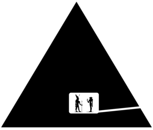
For a random selection of lines through the pyramid, you are also given the total mass of pyramid along that line (this is lower than expected when the line passes through cavities in the pyramid). From this information, you can reconstruct a map of the interior portions of the pyramid using numerical integration. The best map was produced by James Taylor, who won the 2017 Best Student prize:
Note that in 2017, a team of physicists used muon scattering to find a previously unknown void in Khufu’s pyramid using basically the same mathematics. This is also roughly how CT scans work in medical imaging. - 2017 project #2: CodeBreaker which has an accompanying table of English-language digraph frequencies. In CodeBreaker, you are given the encrypted text
RTQIJQRHNZAQFGJAQFBIBQKRGQXJBFBRRTHDJKHSQRGQXBKWFG ZJJPBAJKRBHKRVGBIGHKJAQMIQEEEJKWFGLZJQPFGQKPFGBIDK JRRQKPBRQEVQMRPJSBKQLEJLMZJSJZJKIJFHFGZJJTEQKJRJQI GQFZBWGFQKWEJRFHFGJHFGJZRLNFRHAJTGBEHRHTGBIQETJHTE JGQXJLJJKQRDBKWVGMFGZJJPBAJKRBHKRTQZFBINEQZEMVGMKH FQKHFGJZPBZJIFBHKQFZBWGFQKWEJRFHFGJHFGJZFGZJJQKPGQ XJJXJKFZBJPFHIHKRFZNIFQSHNZPBAJKRBHKWJHAJFZMTZHSJR RHZRBAHKKJVIHALVQRJYTHNKPBKWFGBRFHFGJKJVMHZDAQFGJA QFBIQERHIBJFMHKEMQAHKFGHZRHQWHMHNDKHVGHVHKQSEQFRNZ SQIJVGBIGGQRHKEMFVHPBAJKRBHKRVJIQKZJTZJRJKFQSBWNZJ HSQFGZJJPBAJKRBHKQERHEBPQKPRBABEQZEMFGJMFGBKDFGQFL MAHPJERHSFGZJJPBAJKRBHKRFGJMIHNEPZJTZJRJKFHKJHSSHN ZBSFGJMIHNEPAQRFJZFGJTJZRTJIFBXJHSFGJFGBKWRJJBFGBK DRHANZANZJPFGJTZHXBKIBQEAQMHZQKPDKBFFBKWGBRLZHVRGJ EQTRJPBKFHQKBKFZHRTJIFBXJRFQFJGBREBTRAHXBKWQRHKJVG HZJTJQFRAMRFBIVHZPRMJRBFGBKDBRJJBFKHVGJRQBPQSFJZRH AJFBAJLZBWGFJKBKWBKQONBFJFZQKRBFHZMAQKKJZVJEEBPHKH FABKPFJEEBKWMHNBGQXJLJJKQFVHZDNTHKFGBRWJHAJFZMHSSH NZPBAJKRBHKRSHZRHAJFBAJRHAJHSAMZJRNEFRQZJINZBHNRSH ZBKRFQKIJGJZJBRQTHZFZQBFHSQAQKQFJBWGFMJQZRHEPQKHFG JZQFSBSFJJKQKHFGJZQFRJXJKFJJKQKHFGJZQFFVJKFMFGZJJQ KPRHHKQEEFGJRJQZJJXBPJKFEMRJIFBHKRQRBFVJZJFGZJJPBA JKRBHKQEZJTZJRJKFQFBHKRHSGBRSHNZPBAJKRBHKJPLJBKWVG BIGBRQSBYJPQKPNKQEFJZQLEJFGBKWRIBJKFBSBITJHTEJTZHI JJPJPFGJFBAJFZQXJEEJZQSFJZFGJTQNRJZJONBZJPSHZFGJTZ HTJZQRRBABEQFBHKHSFGBRDKHVXJZMVJEEFGQFFBAJBRHKEMQD BKPHSRTQIJGJZJBRQTHTNEQZRIBJKFBSBIPBQWZQAQVJQFGJZZ JIHZPFGBREBKJBFZQIJVBFGAMSBKWJZRGHVRFGJAHXJAJKFHSF GJLQZHAJFJZMJRFJZPQMBFVQRRHGBWGMJRFJZPQMKBWGFBFSJE EFGJKFGBRAHZKBKWBFZHRJQWQBKQKPRHWJKFEMNTVQZPFHGJZJ RNZJEMFGJAJZINZMPBPKHFFZQIJFGBREBKJBKQKMHSFGJPBAJK RBHKRHSRTQIJWJKJZQEEMZJIHWKBCJPLNFIJZFQBKEMBFFZQIJ PRNIGQEBKJQKPFGQFEBKJFGJZJSHZJVJANRFIHKIENPJVQRQEH KWFGJFBAJPBAJKRBHK
and asked to automatically decrypt it by using optimization to match frequencies of letters and pairs of letters in English text.
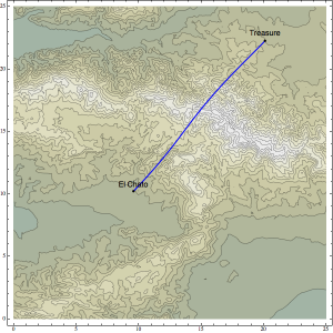
- 2013 project: Taco-Related Mountain Navigation Challenge, and TerrainPackage.m along with TerrainPackageTester.nb.
In the TRMNC, you are given a function z(x,y) describing the topography of the L.A. basin and are asked to find the shortest overland route between the “El Chato” taco truck and a set of coordinates in the desert.
The 2013 winner was Scott Barnes, whose Bezier curve solution is shown below. This solution has length 16.403 km, which is the new number to beat. Congratulations, Scott!


Extra class resources.
I’ve compiled some extra lectures and demonstrations from past versions of the class. I’m not going to cover these in the current class, but I’d like to leave them available to you for further reading.
- Numerical differentiation with noise. Numerical Differentiation of Noisy, Nonsmooth Data by Chartrand. The second is a demonstration of Chartrand’s method.
- Computing Derivatives of Polylines. This lecture is based on the paper Asymptotic Analysis of Discrete Normals and Curvatures of Polylines. These methods are implemented in curvature and torsion of polylines with the data set trefoil data.dat.
- Gauss Quadrature. Another integration rule, which is based on the Legendre polynomials.
- Newton-Cotes Rules. This lecture is different from the others because the entire lecture is given in Mathematica.
- The trapezoid rule for periodic functions and Clenshaw-Curtis quadrature.
- Adaptive Integration and Simpson’s Rule. This doesn’t have a demonstration (yet).
- Minimization with derivatives. If you can compute derivatives of your function symbolically (this can be a big if in applications!) you can do somewhat better than just using a straight Brent’s method. See Section 10.3 of Numerical Recipes in C (Press, Flannery, Teukolsky, Vetterling) and our Mathematica implementation of Brent’s method with derivatives.
Material on this page is a work-for-hire produced for the University of Georgia.